Re可変PINNで複数のレイノルズ数を一度に学習する|パラメトリックPINNの実装

前回の記事では、 固定のキャビティ流れをPINNで解きました。今回は、レイノルズ数 を入力パラメータに加えたパラメトリックPINNに挑戦します。一つのニューラルネットワークで の範囲の流れを同時に学習し、学習後は任意の に対して流れ場を即座に予測できるようにします。記事の一番下に今回のコード全体を乗せています。
パラメトリックPINNとは何か
通常のPINNの課題
通常のPINNでは、 などの物理パラメータは固定値としてネットワークを学習します。異なる の流れを調べたい場合、その都度ネットワークを再学習する必要があります。これは計算コストの観点から非効率です。
Re数を入力に加えるアプローチ
パラメトリックPINNでは、物理パラメータ(今回は )をニューラルネットワークの入力に追加します。これにより、一度の学習で複数のパラメータ値に対応した解を獲得できます。学習済みモデルは、学習範囲内の任意の に対して瞬時に流れ場を予測できるサロゲートモデルとして機能します。
問題設定|キャビティ流れとReの範囲
キャビティ流れ
キャビティ流れは、四方を壁に囲まれた正方形領域の上辺だけが一定速度で移動する流れです。上辺の移動によってキャビティ内部に渦が形成されます。幾何形状がシンプルで境界条件が明確なため、数値計算手法の検証用ベンチマーク問題として広く使われます。
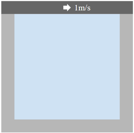
今回の計算条件は以下のとおりです。
| パラメータ | 値 |
|---|---|
| 領域サイズ | |
| 上辺の移動速度 | |
| 流体密度 | |
| レイノルズ数 | (学習範囲) |
| 動粘性係数 | (Reに依存) |
が小さいほど粘性力が支配的になり、大きいほど慣性力が支配的になります。 の範囲では、いずれも定常な渦構造が形成されますが、渦の形状や強度は によって変化します。
支配方程式とRe数の扱い方
定常非圧縮Navier-Stokes方程式
今回は定常・非圧縮の流れとします。したがって支配方程式は連続の式と運動量方程式です。
連続の式(質量保存):
方向の運動量方程式:
方向の運動量方程式:
各記号の意味は以下のとおりです。
| 記号 | 意味 |
|---|---|
| 方向、方向の速度成分 | |
| 圧力 | |
| 密度 | |
| 動粘性係数 |
方程式でのRe数の扱い方
パラメトリックPINNでは、方程式中の を として、 を記号(シンボル)として扱います。これにより、学習時に様々な 値で方程式の残差を計算できます。
physicsnemoでは、SymPyの Symbol を使って を記号変数として定義します:
from sympy import Symbol

eq = NavierStokes(nu=1 / Symbol("Re"), rho=1.0, dim=2)
この方法により、PhysicsInformer がPDE残差を計算する際に、その時点で指定された 値を使って残差を評価できます。
境界条件
境界条件は以下のとおりです。
| 境界 | 条件 |
|---|---|
| 上辺(移動壁) | 、 |
| その他の壁(左・右・下辺) | 、(滑りなし条件) |
形状とデータローダーの設定
形状の定義
形状の定義には physicsnemo.sym.geometry.primitives_2d.Rectangle クラスを使用します。以下の例では、キャビティの中心を原点とし、 の正方形領域を作成しています。
from physicsnemo.sym.geometry.primitives_2d import Rectangle

class Cavity:
    def __init__(self, dim=2, length=1.0):
        self.dim = dim
        self.length = length

        p1 = (-length / 2, -length / 2)
        p2 = (length / 2, length / 2)
        self.interior = Rectangle(point_1=p1, point_2=p2)
physicsnemoには、Rectangle のほかにも基本的な形状を作成するためのクラスが用意されています。形状クラスは内部と表面のサンプリング機能を持ち、次の GeometryDatapipe と組み合わせることで境界点・内部点を自動的に生成できます。
コロケーション点のサンプリング方法|GeometryDatapipe
損失関数の計算には、各学習ステップで形状の内部と表面から点をサンプルする必要があります。サンプリングにはphysicsnemoの GeometryDatapipe を使用します。
from physicsnemo.sym.geometry.geometry_dataloader import GeometryDatapipe

def create_geometry_dataloader(geom_object, batch_size, num_points, sample_type, requested_vars):
    return GeometryDatapipe(
        geom_objects=[geom_object],
        batch_size=batch_size,
        num_points=num_points,
        sample_type=sample_type,
        device=device,
        num_workers=1,
        requested_vars=requested_vars,
    )

geo = Cavity(dim=2, length=cavity_length)
boundary_dl = create_geometry_dataloader(geo.interior, 1, 4000, "surface", ["x", "y"])
interior_dl = create_geometry_dataloader(geo.interior, 1, 10000, "volume", ["x", "y", "sdf"])
sample_type="surface" は境界から点をサンプリングし、sample_type="volume" は内部からサンプリングします。内部点のサンプリングでは SDF(符号付き距離関数)も取得できます。SDFは各点から最寄りの壁面までの距離で、PDE損失の重みとして利用します。
今回はサンプリング点数を表面から4,000点、内部から10,000点としました。パラメトリックPINNでは の範囲全体を学習する必要があるため、通常のPINNよりも多めに設定しています。
ニューラルネットワークの設計|3入力・3出力の構成
ニューラルネットワーク(NN)には全結合層を積み重ねた多層パーセプトロンを使用します。physicsnemoでは、PyTorchと同じ方法でNNを定義できます。
import torch.nn as nn

class CustomFullyConnected(nn.Module):
    def __init__(
        self,
        in_features: int = 512,
        out_features: int = 512,
        layer_size: int = 512,
        num_layers: int = 6,
        softplus: bool = False,
    ):
        super().__init__()
        self.softplus = softplus
        self.layers = nn.ModuleList()

        layers_in_features = in_features
        for _ in range(num_layers):
            self.layers.append(nn.Linear(layers_in_features, layer_size))
            self.layers.append(nn.SiLU())
            layers_in_features = layer_size

        self.final_layer = nn.Linear(layer_size, out_features, bias=True)

    def forward(self, x):
        for layer in self.layers:
            x = layer(x)
        x = self.final_layer(x)
        if self.softplus:
            x = nn.Softplus()(x)
        return x
通常のPINNとの違いは入力次元です。通常のPINNでは入力が の2次元でしたが、パラメトリックPINNでは を追加して の3次元になります。
| パラメータ | 通常のPINN | パラメトリックPINN |
|---|---|---|
| 入力次元 | 2(, ) | 3(, , ) |
| 出力次元 | 3(, , ) | 3(, , ) |
| 隠れ層のニューロン数 | 256 | 256 |
| 隠れ層の数 | 4 | 4 |
| 活性化関数 | SiLU | SiLU |
# パラメトリックPINN: x, y, Re の3入力
flow_model = CustomFullyConnected(
    in_features=3, out_features=3, num_layers=4, layer_size=256
).to(device)
NN は座標 と正規化された を受け取り、その条件における速度成分 、 と圧力 を出力します。活性化関数にSiLU(Sigmoid Linear Unit、)を採用しています。SiLUは勾配消失が起きにくい特性を持ちます。PINNでは勾配消失が起きると方程式の残差を計算できなくなるため、こうした活性化関数の選択が重要です。
パラメトリックPINNの学習方法|Re数のランダムサンプリング
オプティマイザとスケジューラ
physicsnemoでは、PyTorchのオプティマイザとスケジューラをそのまま利用できます。
optimizer = torch.optim.Adam(flow_model.parameters(), lr=1e-3)
scheduler = torch.optim.lr_scheduler.LambdaLR(
    optimizer, lr_lambda=lambda step: 0.9999**step
)
オプティマイザはAdamを使用し、初期学習率は です。学習率は各ステップごとに 倍に減衰するスケジューラを設定しています。
PhysicsInformerの設定
PhysicsInformerはphysicsnemoが提供するPDE残差の計算モジュールです。方程式クラスと grad_method="autodiff" を指定することで、自動微分によるPDE残差の計算を担います。
パラメトリックPINNでは、 を記号変数として方程式を定義します:
from sympy import Symbol
from physicsnemo.sym.eq.phy_informer import PhysicsInformer

eq = NavierStokes(nu=1 / Symbol("Re"), rho=1.0, dim=2)
phy_inf = PhysicsInformer(
    required_outputs=["continuity", "momentum_x", "momentum_y"],
    equations=eq,
    grad_method="autodiff",
    device=device,
)
Symbol("Re") を使うことで、学習時に動的に 値を渡してPDE残差を計算できるようになります。
学習ループ全体
パラメトリックPINNの学習コードを示します。通常のPINNとの主な違いは、各学習ステップで をランダムにサンプリングし、正規化した をNNに入力する点です。
Re_range = (10, 100)  # 学習するReの範囲
num_steps = 50000
step = 0

for boundary_pts, interior_pts in zip(boundary_dl, interior_dl):
    if step >= num_steps:
        break

    optimizer.zero_grad()

    # 各ステップでReをランダムにサンプリング
    Re = Re_range[0] + np.random.rand() * (Re_range[1] - Re_range[0])
    Re_norm = Re / Re_range[1]  # NNへの入力は正規化されたRe

    # 境界点の入力を作成: (x, y, Re_norm)
    boundary_xy = torch.cat([boundary_pts[0][c].reshape(-1, 1) for c in ["x", "y"]], dim=1)
    boundary_Re = torch.full_like(boundary_xy[:, 0:1], Re_norm, device=device)
    boundary_inputs = torch.cat([boundary_xy, boundary_Re], dim=1)

    topwall_inputs = boundary_inputs[boundary_pts[0]["y"].reshape(-1) == cavity_length / 2]
    otherwall_inputs = boundary_inputs[boundary_pts[0]["y"].reshape(-1) != cavity_length / 2]

    # 内部点の入力を作成: (x, y, Re_norm)
    interior_xy = torch.cat([interior_pts[0][c].reshape(-1, 1) for c in ["x", "y"]], dim=1).requires_grad_(True)
    interior_Re = torch.full_like(interior_xy[:, 0:1], Re_norm, device=device)
    interior_inputs = torch.cat([interior_xy, interior_Re], dim=1)
    sdf = interior_pts[0]["sdf"].reshape(-1, 1)

    # NNで予測
    flow_topwall_out = flow_model(topwall_inputs)
    flow_otherwall_out = flow_model(otherwall_inputs)
    flow_interior_out = flow_model(interior_inputs)

    # 境界条件の損失
    topwall_weighting = 1 - 2 * torch.abs(topwall_inputs[:, 0:1])
    bc_loss = {
        "topwall_u":   torch.mean(topwall_weighting * (flow_topwall_out[:, 0:1] - u_top) ** 2),
        "topwall_v":   torch.mean(topwall_weighting * (flow_topwall_out[:, 1:2]) ** 2),
        "otherwall_u": torch.mean(flow_otherwall_out[:, 0:1] ** 2),
        "otherwall_v": torch.mean(flow_otherwall_out[:, 1:2] ** 2),
    }

    # PDE残差を計算(PhysicsInformerには正規化前のRe値を渡す)
    interior_Re_raw = torch.full_like(interior_Re, Re, device=device)
    pde_out = phy_inf.forward({
        "coordinates": interior_xy,
        "u": flow_interior_out[:, 0:1],
        "v": flow_interior_out[:, 1:2],
        "p": flow_interior_out[:, 2:3],
        "Re": interior_Re_raw,
    })
    pde_loss = {
        k: torch.mean(sdf * pde_out[k] ** 2)
        for k in ["continuity", "momentum_x", "momentum_y"]
    }

    loss = sum(bc_loss.values()) + sum(pde_loss.values())
    loss.backward()
    optimizer.step()
    scheduler.step()
    step += 1
Re数の正規化とPhysicsInformerへの渡し方
をNNに入力する際、正規化が重要です。今回は として の範囲に正規化しています。
Re_norm = Re / Re_range[1] # Re_range = (10, 100) なので、Re_norm ∈ [0.1, 1.0]
正規化する理由は以下のとおりです:
- 入力スケールの統一: 座標 に対して、 などは桁が大きく異なります。スケールを揃えることで学習が安定します
- 勾配のバランス: 入力の大きさが揃っていないと、特定の入力に対する勾配が支配的になり、学習が偏る可能性があります
注意点として、PhysicsInformerには正規化前の実際の 値を渡します。方程式中の が物理量として正しい値を取る必要があるためです。NNへの入力は正規化した値、物理方程式には実際の値、という使い分けが必要です。
境界条件の重み付け
損失関数の工夫として、移動壁の損失を重み付けしています。
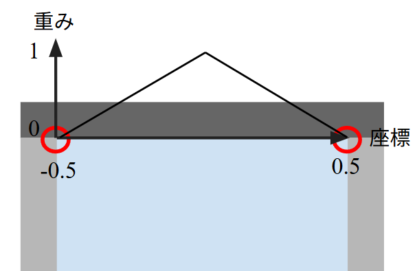
topwall_weighting = 1 - 2 * torch.abs(topwall_inputs[:, 0:1])
bc_loss = {
    "topwall_u":   torch.mean(topwall_weighting * (flow_topwall_out[:, 0:1] - u_top) ** 2),
    ...
}
を移動壁の損失に掛けることで、静止壁に近づくと重みが小さくなるように工夫しています。キャビティ流れのコーナー部分では流速 の境界条件が0から1に不連続に変化します。損失を同じ重みにすると学習が遅くなったり失敗することがあり、位置によって重みを調節することで学習を安定させています。詳細はPINNの学習失敗談の記事で解説しています。
学習結果|Re=10〜100での速度プロファイル比較
PINNの理論と照らし合わせながら結果を確認します。
異なるRe数での流れ場予測
以下の図は、学習したモデルで の流れ場を予測した結果です。一つのモデルで異なる の流れを表現できていることがわかります。
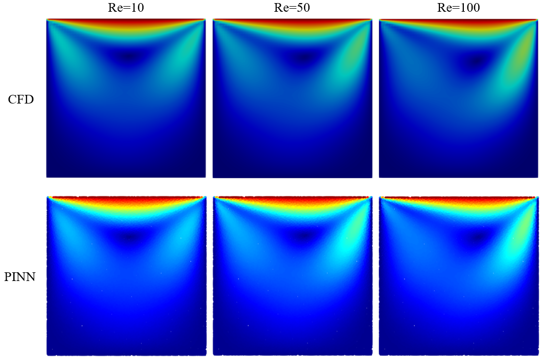
が大きくなるにつれて、主渦の中心位置が右に移動し、渦の強度(速度勾配)が増加するという流れ場の変化を、PINNが正しく学習できています。
速度プロファイルの比較
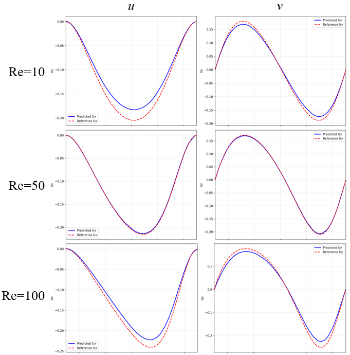
キャビティ中央の垂直線()上での と のプロファイルを示します。異なる に対して、PINNの予測とCFD解を比較しています。青実線がPINNの予測値、赤破線が参照解(CFD)です。Reが大きくなると主渦が右に移動する傾向は学習できています。一方で、流速のピーク値は で誤差が大きくなっています。
境界付近で精度が落ちる原因と改善策
では精度が良く、学習範囲の上下限である で誤差が大きくなった原因は、NNが入力範囲の境界付近の学習を苦手とする傾向があるためと考えられます。NNは学習データ全体から平均的なパターンを学習しようとするため、範囲の中央付近(今回は )では周囲の学習データから補間的に予測できます。一方、境界付近()では片側からしか情報が得られず、外挿的な要素が入りやすくなります。
この原因が正しければ、以下のアプローチによって精度が改善すると期待できます:
- 重点サンプリング: の境界付近( 近傍)でより多くサンプリングする
- 学習範囲の拡大: が境界にならないよう、 などに学習範囲を広げる
まとめ|パラメトリックPINNの実装ポイント
physicsnemoを使って、 を入力パラメータに含めたパラメトリックPINNを実装しました。通常のPINNとの主な違いは以下の3点です:
| 項目 | 通常のPINN | パラメトリックPINN |
|---|---|---|
| NN入力 | ||
| 方程式中の | (定数) | (記号) |
| 学習時の | 固定値 | 各ステップでランダムサンプリング |
実装のポイントをまとめると:
- NN入力の正規化: は で割って正規化し、座標とスケールを揃える
- PhysicsInformerには実際の 値を渡す: 物理方程式では正規化前の値が必要
- SymPyの
Symbolで記号変数を定義: 学習時に動的に を変更可能にする
パラメトリックPINNは、学習後に任意の で即座に流れ場を予測できるため、設計パラメータの探索やリアルタイムシミュレーションに応用できます。
コード全体
geometry.py
from physicsnemo.sym.geometry.primitives_2d import Rectangle


class Cavity:
    def __init__(self, dim=2, length=1.0):
        self.dim = dim
        self.length = length

        p1 = (-length / 2, -length / 2)
        p2 = (length / 2, length / 2)
        self.interior = Rectangle(point_1=p1, point_2=p2)
model.py
import torch.nn as nn


class CustomFullyConnected(nn.Module):
    def __init__(
        self,
        in_features: int = 512,
        out_features: int = 512,
        layer_size: int = 512,
        num_layers: int = 6,
        softplus: bool = False,
    ):
        super().__init__()
        self.softplus = softplus
        self.layers = nn.ModuleList()

        layers_in_features = in_features
        for _ in range(num_layers):
            self.layers.append(nn.Linear(layers_in_features, layer_size))
            self.layers.append(nn.SiLU())
            layers_in_features = layer_size

        self.final_layer = nn.Linear(layer_size, out_features, bias=True)

    def forward(self, x):
        for layer in self.layers:
            x = layer(x)
        x = self.final_layer(x)
        if self.softplus:
            x = nn.Softplus()(x)
        return x
eq.py
方程式クラスです。physicsnemoの PDE クラスを継承し、SymPyで方程式を定義します。各偏微分はSymPyの .diff() で記述し、PhysicsInformer が自動微分でこれらの残差を計算します。パラメトリックPINNでは、nu を記号変数として受け取れるようにしています。
from sympy import Symbol, Function, Number, simplify
from physicsnemo.sym.eq.pde import PDE


class NavierStokes(PDE):
    def __init__(self, nu=1, rho=1, dim=2):
        if isinstance(nu, (int, float)):
            nu = Number(nu)
        if isinstance(rho, (int, float)):
            rho = Number(rho)

        x, y = Symbol("x"), Symbol("y")
        u = Function("u")(x, y)
        v = Function("v")(x, y)
        p = Function("p")(x, y)

        self.equations = {
            "continuity": simplify(u.diff(x) + v.diff(y)),
            "momentum_x": simplify(
                u * u.diff(x) + v * u.diff(y)
                + (1 / rho) * p.diff(x)
                - nu * (u.diff(x, 2) + u.diff(y, 2))
            ),
            "momentum_y": simplify(
                u * v.diff(x) + v * v.diff(y)
                + (1 / rho) * p.diff(y)
                - nu * (v.diff(x, 2) + v.diff(y, 2))
            ),
        }
train.py
import numpy as np
import torch
from sympy import Symbol
from physicsnemo.sym.eq.phy_informer import PhysicsInformer
from physicsnemo.sym.geometry.geometry_dataloader import GeometryDatapipe

from eq import NavierStokes
from geometry import Cavity
from model import CustomFullyConnected

device = "cuda:0" if torch.cuda.is_available() else "cpu"

Re_range = (10, 100)  # 学習するReの範囲
u_top = 1.0
cavity_length = 1.0

# Reを記号変数として方程式を定義
eq = NavierStokes(nu=1 / Symbol("Re"), rho=1.0, dim=2)
phy_inf = PhysicsInformer(
    required_outputs=["continuity", "momentum_x", "momentum_y"],
    equations=eq,
    grad_method="autodiff",
    device=device,
)

geo = Cavity(dim=2, length=cavity_length)
boundary_dl = GeometryDatapipe(
    geom_objects=[geo.interior], batch_size=1, num_points=4000,
    sample_type="surface", device=device, num_workers=1,
    requested_vars=["x", "y"],
)
interior_dl = GeometryDatapipe(
    geom_objects=[geo.interior], batch_size=1, num_points=10000,
    sample_type="volume", device=device, num_workers=1,
    requested_vars=["x", "y", "sdf"],
)

# パラメトリックPINN: 入力次元が3 (x, y, Re)
flow_model = CustomFullyConnected(
    in_features=3, out_features=3, num_layers=4, layer_size=256
).to(device)

optimizer = torch.optim.Adam(flow_model.parameters(), lr=1e-3)
scheduler = torch.optim.lr_scheduler.LambdaLR(
    optimizer, lr_lambda=lambda step: 0.9999**step
)

num_steps = 50000
step = 0
for boundary_pts, interior_pts in zip(boundary_dl, interior_dl):
    if step >= num_steps:
        break
    optimizer.zero_grad()

    # 各ステップでReをランダムサンプリング
    Re = Re_range[0] + np.random.rand() * (Re_range[1] - Re_range[0])
    Re_norm = Re / Re_range[1]  # 正規化

    # 境界点の入力作成
    boundary_xy = torch.cat([boundary_pts[0][c].reshape(-1, 1) for c in ["x", "y"]], dim=1)
    boundary_Re = torch.full_like(boundary_xy[:, 0:1], Re_norm, device=device)
    boundary_inputs = torch.cat([boundary_xy, boundary_Re], dim=1)
    topwall_inputs = boundary_inputs[boundary_pts[0]["y"].reshape(-1) == cavity_length / 2]
    otherwall_inputs = boundary_inputs[boundary_pts[0]["y"].reshape(-1) != cavity_length / 2]

    # 内部点の入力作成
    interior_xy = torch.cat([interior_pts[0][c].reshape(-1, 1) for c in ["x", "y"]], dim=1).requires_grad_(True)
    interior_Re = torch.full_like(interior_xy[:, 0:1], Re_norm, device=device)
    interior_inputs = torch.cat([interior_xy, interior_Re], dim=1)
    sdf = interior_pts[0]["sdf"].reshape(-1, 1)

    flow_topwall_out = flow_model(topwall_inputs)
    flow_otherwall_out = flow_model(otherwall_inputs)
    flow_interior_out = flow_model(interior_inputs)

    topwall_weighting = 1 - 2 * torch.abs(topwall_inputs[:, 0:1])
    bc_loss = {
        "topwall_u":   torch.mean(topwall_weighting * (flow_topwall_out[:, 0:1] - u_top) ** 2),
        "topwall_v":   torch.mean(topwall_weighting * (flow_topwall_out[:, 1:2]) ** 2),
        "otherwall_u": torch.mean(flow_otherwall_out[:, 0:1] ** 2),
        "otherwall_v": torch.mean(flow_otherwall_out[:, 1:2] ** 2),
    }

    # PhysicsInformerには実際のRe値を渡す
    interior_Re_raw = torch.full_like(interior_Re, Re, device=device)
    pde_out = phy_inf.forward({
        "coordinates": interior_xy,
        "u": flow_interior_out[:, 0:1],
        "v": flow_interior_out[:, 1:2],
        "p": flow_interior_out[:, 2:3],
        "Re": interior_Re_raw,
    })
    pde_loss = {
        k: torch.mean(sdf * pde_out[k] ** 2)
        for k in ["continuity", "momentum_x", "momentum_y"]
    }

    loss = sum(bc_loss.values()) + sum(pde_loss.values())
    loss.backward()
    optimizer.step()
    scheduler.step()
    step += 1
さらに深く学ぶための書籍
本記事のテーマをより深く学びたい方には、以下の書籍をおすすめします。
入門・学部レベル
- ゼロから作るDeepLearning(斎藤康毅、オライリー・ジャパン):ニューラルネットワークと自動微分の仕組みをゼロから実装しながら学べる一冊です。Physics Informedについての記述はありませんが、行間が丁寧で分かりやすく、ニューラルネットワークの学習を深く理解するには非常に役立ちます。
発展・大学院レベル
- Data-Driven Science and Engineering: Machine Learning, Dynamical Systems, and Control(Steven L. Brunton・J. Nathan Kutz、Cambridge University Press):データ駆動型の流体力学・物理シミュレーションを体系的に解説しており、PINNを含む最新手法を学ぶのに適した一冊です。
参考文献
- M. Raissi, P. Perdikaris, G.E. Karniadakis, "Physics-informed neural networks: A deep learning framework for solving forward and inverse problems involving nonlinear partial differential equations", Journal of Computational Physics, Vol. 378, pp. 686–707, 2019. DOI: 10.1016/j.jcp.2018.10.045