PINNで2次元キャビティ流れを解く|physicsnemoを使ったNavier-Stokes方程式の求解

Physics Informed Neural Networks(PINN)を用いて、2次元キャビティ流れを解きます。フレームワークにはNVIDIAのphysicsnemoを使用します。この記事では、Physics Informed Neural Networks (PINN)とは?で解説したPINNの基礎的な理論を、Navier-Stokes方程式に適用する場合どう実装するかを分かりやすく解説します。記事の一番下に今回のコード全体を乗せてます。
問題設定
キャビティ流れとは
キャビティ流れは、四方を壁に囲まれた正方形領域の上辺だけが一定速度で移動する流れです。上辺の移動によってキャビティ内部に渦が形成されます。幾何形状がシンプルで境界条件が明確なため、数値計算手法の検証用ベンチマーク問題として広く使われます。
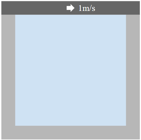
今回の計算条件は以下のとおりです。
| パラメータ | 値 |
|---|---|
| 領域サイズ | |
| 上辺の移動速度 | |
| 流体密度 | |
| レイノルズ数 | |
| 動粘性係数 |
は粘性力が支配的な低レイノルズ数領域に相当し、定常な一渦構造が形成されます。
方程式
定常非圧縮Navier-Stokes方程式
今回は定常・非圧縮の流れとします。したがって支配方程式は連続の式と運動量方程式です。
連続の式(質量保存):
方向の運動量方程式:
方向の運動量方程式:
各記号の意味は以下のとおりです。
| 記号 | 意味 |
|---|---|
| 方向、方向の速度成分 | |
| 圧力 | |
| 密度 | |
| 動粘性係数 |
PINNでは、これら3式の残差を損失関数に組み込みます。
境界条件
境界条件は以下のとおりです。
| 境界 | 条件 |
|---|---|
| 上辺(移動壁) | 、 |
| その他の壁(左・右・下辺) | 、(滑りなし条件) |
形状
形状の定義には physicsnemo.sym.geometry.primitives_2d.Rectangle クラスを使用します。以下の例では、キャビティの中心を原点とし、 の正方形領域を作成しています。
from physicsnemo.sym.geometry.primitives_2d import Rectangle

class Cavity:
    def __init__(self, dim=2, length=1.0):
        self.dim = dim
        self.length = length

        p1 = (-length / 2, -length / 2)
        p2 = (length / 2, length / 2)
        self.interior = Rectangle(point_1=p1, point_2=p2)
physicsnemoには、Rectangle のほかにも基本的な形状を作成するためのクラスが用意されています。形状を作成するクラス(正確には physicsnemo.sym.geometry.geometry.Geometry を継承したクラス)は、形状の内部と表面のサンプリング機能を持ちます。次の GeometryDatapipe と組み合わせることで、境界点・内部点を自動的に生成できます。
データローダー
GeometryDatapipe
損失関数の計算には、各学習ステップで形状の内部と表面から点をサンプルする必要がありました。サンプリングにはphysicsnemoの physicsnemo.sym.geometry.geometry_dataloader.GeometryDatapipe を使用します。
from physicsnemo.sym.geometry.geometry_dataloader import GeometryDatapipe

def create_geometry_dataloader(geom_object, batch_size, num_points, sample_type, requested_vars):
    return GeometryDatapipe(
        geom_objects=[geom_object],
        batch_size=batch_size,
        num_points=num_points,
        sample_type=sample_type,
        device=device,
        num_workers=1,
        requested_vars=requested_vars,
    )

geo = Cavity(dim=2, length=cavity_length)
wall_dl   = create_geometry_dataloader(geo.interior, 1, 2000,  "surface", ["x", "y"])
interior_dl = create_geometry_dataloader(geo.interior, 1, 10000, "volume",  ["x", "y", "sdf"])
sample_type="surface" はgeom_objectsの表面(境界)から点をサンプリングします。sample_type="volume" はgeom_objectsの内部からサンプリングします。
内部点のサンプリングでは SDF(符号付き距離関数、Signed Distance Function)も取得できます。SDFは各点から最寄りの壁面までの距離を表しており、PINNではこのSDFをPDE損失の重みとして利用することがあります。(詳細は学習セクションで説明)。
今回はサンプリング点数を表面から2,000点、内部から10,000点としました。
ニューラルネットワーク
ニューラルネットワーク(NN)には全結合層を積み重ねた多層パーセプトロンを使用します。physicsnemoでは、pytorchと同じ方法でNNを定義できます。
import torch.nn as nn

class CustomFullyConnected(nn.Module):
    def __init__(
        self,
        in_features: int = 512,
        out_features: int = 512,
        layer_size: int = 512,
        num_layers: int = 6,
        softplus: bool = False,
    ):
        super().__init__()
        self.softplus = softplus
        self.layers = nn.ModuleList()

        layers_in_features = in_features
        for _ in range(num_layers):
            self.layers.append(nn.Linear(layers_in_features, layer_size))
            self.layers.append(nn.SiLU())
            layers_in_features = layer_size

        self.final_layer = nn.Linear(layer_size, out_features, bias=True)

    def forward(self, x):
        for layer in self.layers:
            x = layer(x)
        x = self.final_layer(x)
        if self.softplus:
            x = nn.Softplus()(x)
        return x
今回の使用条件は以下のとおりです。
| パラメータ | 値 |
|---|---|
| 入力次元 | 2(, 座標) |
| 出力次元 | 3(, , ) |
| 隠れ層のニューロン数 | 256 |
| 隠れ層の数 | 4 |
| 活性化関数 | SiLU |
flow_model = CustomFullyConnected(
    in_features=2, out_features=3, num_layers=4, layer_size=256
).to(device)
NN は座標 を受け取り、その点における速度成分 、 と圧力 を同時に出力します。そのため in_features=2 、 out_features=3 としました。活性化関数にSiLU(Sigmoid Linear Unit)を採用しています。SiLUは で定義され、勾配消失が起きにくい特性を持ちます。PINNでは勾配消失が起きると方程式の残差を計算できなくなるため、こうした勾配消失しにくい活性化関数を選ぶことが重要です。
学習条件
オプティマイザとスケジューラ
physicsnemoでは、pytorchのオプティマイザとスケジューラをそのまま利用できます。
optimizer = torch.optim.Adam(flow_model.parameters(), lr=1e-3)
scheduler = torch.optim.lr_scheduler.LambdaLR(
    optimizer, lr_lambda=lambda step: 0.9999**step
)
オプティマイザはAdamを使用し、初期学習率は です。学習率は各ステップごとに 倍に減衰するスケジューラを設定しています。
PhysicsInformer
PhysicsInformerはphysicsnemoが提供するPDE残差の計算モジュールです。方程式クラスと grad_method="autodiff" を指定することで、自動微分によるPDE残差の計算を担います。
方程式クラスはphysicsnemoの PDE クラスを継承して定義します。以下の例では、Navier-Stokes方程式の残差を計算するPhysicsInformerクラスを定義しています。
from physicsnemo.sym.eq.phy_informer import PhysicsInformer

eq = NavierStokes(nu=1 / Re, rho=1.0, dim=2)
phy_inf = PhysicsInformer(
    required_outputs=["continuity", "momentum_x", "momentum_y"],
    equations=eq,
    grad_method="autodiff",
    device=device,
)
NavierStokes クラスには定常非圧縮Navier-Stokes方程式(連続の式、方向運動量方程式)実装しました。詳細はコード全体のセクションで確認できます。
学習
学習コードを示します。
num_steps = 10000
step = 0

def stack_coords(pts_dict):
    return torch.cat([pts_dict[0][c].reshape(-1, 1) for c in ["x", "y"]], dim=1)

for wall_pts, interior_pts in zip(wall_dl, interior_dl):  # データローダーで表面2,000点、内部10,000点サンプリング
    if step >= num_steps:
        break

    optimizer.zero_grad()

    wall_points      = stack_coords(wall_pts)  # NNに入力できる形に整形
    topwall_points   = wall_points[wall_pts[0]["y"].reshape(-1) == cavity_length / 2]  # 移動壁だけ取得
    otherwall_points = wall_points[wall_pts[0]["y"].reshape(-1) != cavity_length / 2]  # 移動壁以外を取得

    interior_points  = stack_coords(interior_pts).requires_grad_(True)  # NNに入力できる形に整形
    sdf = interior_pts[0]["sdf"].reshape(-1, 1)  ## あとで損失関数の重み付けに利用

    flow_topwall_out   = flow_model(topwall_points)   # 移動壁におけるu, v, p
    flow_otherwall_out = flow_model(otherwall_points) # 移動壁以外のu, v, p
    flow_interior_out  = flow_model(interior_points)  # 内部のu, v, p

    topwall_weighting = 1 - 2 * torch.abs(topwall_points[:, 0:1])  # 損失関数の重み付けに利用
    # 境界条件の誤差を計算
    bc_loss = {
        "topwall_u":   torch.mean(topwall_weighting * (flow_topwall_out[:, 0:1] - u_top) ** 2),
        "topwall_v":   torch.mean(topwall_weighting * (flow_topwall_out[:, 1:2]) ** 2),
        "otherwall_u": torch.mean(flow_otherwall_out[:, 0:1] ** 2),
        "otherwall_v": torch.mean(flow_otherwall_out[:, 1:2] ** 2),
    }

    # PDE残差を計算
    pde_out = phy_inf.forward({
        "coordinates": interior_points,
        "u": flow_interior_out[:, 0:1],
        "v": flow_interior_out[:, 1:2],
        "p": flow_interior_out[:, 2:3],
    })
    pde_loss = {
        k: torch.mean(2 * sdf * pde_out[k] ** 2)
        for k in ["continuity", "momentum_x", "momentum_y"]
    }

    # Lossを計算、NNの学習パラメータを更新
    loss = sum(bc_loss.values()) + sum(pde_loss.values())
    loss.backward()
    optimizer.step()
    scheduler.step()
    step += 1
PINNの理論と照らし合わせながらコードを読むと、おおよその流れを掴みやすいです。
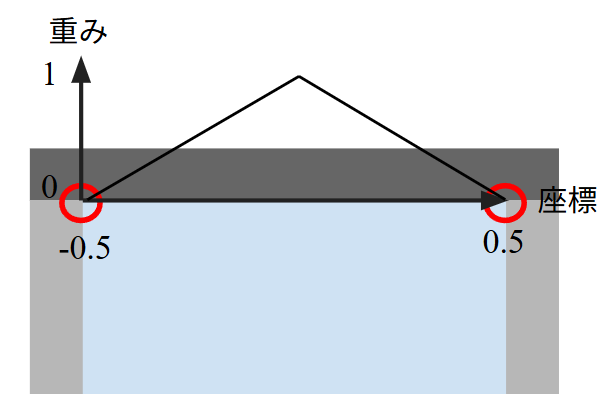
損失関数の工夫として、移動壁の損失を重み付けしています。
    topwall_weighting = 1 - 2 * torch.abs(topwall_points[:, 0:1])  # 損失関数の重み付けに利用
    # 境界条件の誤差を計算
    bc_loss = {
        "topwall_u":   torch.mean(topwall_weighting * (flow_topwall_out[:, 0:1] - u_top) ** 2),
        "topwall_v":   torch.mean(topwall_weighting * (flow_topwall_out[:, 1:2]) ** 2),
        "otherwall_u": torch.mean(flow_otherwall_out[:, 0:1] ** 2),
        "otherwall_v": torch.mean(flow_otherwall_out[:, 1:2] ** 2),
    }
を移動壁の損失に掛けることで、静止壁に近づくと重みが小さくなるように工夫しています。キャビティ流れでは、図の赤丸部分では流速uの境界条件が0から1に不連続に変化します。場に不連続が存在する場合、損失を同じ重みにすると学習が遅くなったり失敗することがあります。このように位置によって重みを調節することで、学習を早めたり、失敗する可能性を下げることができます。
学習結果
PINNの計算結果とCFDの参照解を比較します。
速度の大きさ(全体)
以下の図はキャビティ全体の速度の大きさ()を示します。
左:CFD(参照解)右:PINN
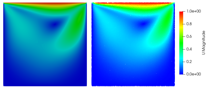
上辺付近で速度が大きく、キャビティ中央にかけて渦を形成している様子が、PINNでも再現されています。
速度プロファイル
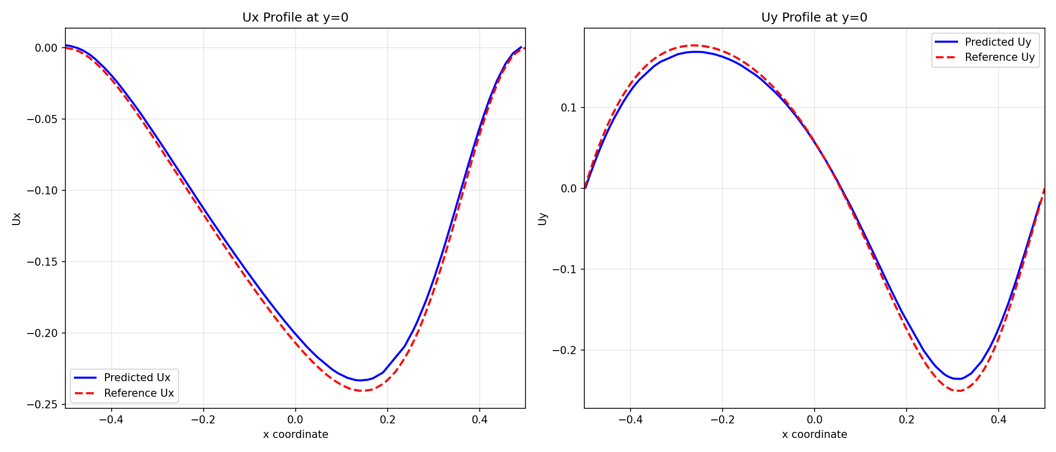
キャビティ中央の垂直線()上での 速度プロファイルと、水平線()上での 速度プロファイルを示します。青線が学習したNNの予測値、赤破線が参照解(CFD結果)です。PINNの結果はCFD解と概ね一致しており、PINNが定常Navier-Stokes方程式を正しく解けています。
まとめ
physicsnemoを使ったPINNで、 の2次元キャビティ流れを解きました。形状や境界条件を変えることで、キャビティ以外の非圧縮流れを解くことができます。 physicsnemoを使う際のポイントとしては、
- PhysicsInformerにより、自動微分を用いたNavier-Stokes方程式の残差計算を実装できます
- SDFを損失重みに使うことで、壁面付近の学習を安定させられます
- コーナーの速度不連続に対しては、重み付き境界条件損失で対処できます
今回は の固定条件で学習しました。次は を入力パラメータに含め、異なるレイノルズ数の流れを一つのNNで表現できるパラメトリックPINNの構築に挑戦します。
コード全体
geometry.py
from physicsnemo.sym.geometry.primitives_2d import Rectangle


class Cavity:
    def __init__(self, dim=2, length=1.0):
        self.dim = dim
        self.length = length

        p1 = (-length / 2, -length / 2)
        p2 = (length / 2, length / 2)
        self.interior = Rectangle(point_1=p1, point_2=p2)
model.py
import torch.nn as nn


class CustomFullyConnected(nn.Module):
    def __init__(
        self,
        in_features: int = 512,
        out_features: int = 512,
        layer_size: int = 512,
        num_layers: int = 6,
        softplus: bool = False,
    ):
        super().__init__()
        self.softplus = softplus
        self.layers = nn.ModuleList()

        layers_in_features = in_features
        for _ in range(num_layers):
            self.layers.append(nn.Linear(layers_in_features, layer_size))
            self.layers.append(nn.SiLU())
            layers_in_features = layer_size

        self.final_layer = nn.Linear(layer_size, out_features, bias=True)

    def forward(self, x):
        for layer in self.layers:
            x = layer(x)
        x = self.final_layer(x)
        if self.softplus:
            x = nn.Softplus()(x)
        return x
eq.py
方程式クラスです。physicsnemoの PDE クラスを継承し、SymPyで方程式を定義します。各偏微分はSymPyの .diff() で記述し、PhysicsInformer が自動微分でこれらの残差を計算します。
from sympy import Symbol, Function, Number, simplify
from physicsnemo.sym.eq.pde import PDE


class NavierStokes(PDE):
    def __init__(self, nu=1, rho=1, dim=2):
        if isinstance(nu, (int, float)):
            nu = Number(nu)
        if isinstance(rho, (int, float)):
            rho = Number(rho)

        x, y = Symbol("x"), Symbol("y")
        u = Function("u")(x, y)
        v = Function("v")(x, y)
        p = Function("p")(x, y)

        self.equations = {
            "continuity": simplify(u.diff(x) + v.diff(y)),
            "momentum_x": simplify(
                u * u.diff(x) + v * u.diff(y)
                + (1 / rho) * p.diff(x)
                - nu * (u.diff(x, 2) + u.diff(y, 2))
            ),
            "momentum_y": simplify(
                u * v.diff(x) + v * v.diff(y)
                + (1 / rho) * p.diff(y)
                - nu * (v.diff(x, 2) + v.diff(y, 2))
            ),
        }
train.py
import torch
from physicsnemo.sym.eq.phy_informer import PhysicsInformer
from physicsnemo.sym.geometry.geometry_dataloader import GeometryDatapipe

from eq import NavierStokes
from geometry import Cavity
from model import CustomFullyConnected

device = "cuda:0" if torch.cuda.is_available() else "cpu"

Re = 100
u_top = 1.0
cavity_length = 1.0

eq = NavierStokes(nu=1 / Re, rho=1.0, dim=2)
phy_inf = PhysicsInformer(
    required_outputs=["continuity", "momentum_x", "momentum_y"],
    equations=eq,
    grad_method="autodiff",
    device=device,
)

geo = Cavity(dim=2, length=cavity_length)
wall_dl = GeometryDatapipe(
    geom_objects=[geo.interior], batch_size=1, num_points=2000,
    sample_type="surface", device=device, num_workers=1,
    requested_vars=["x", "y"],
)
interior_dl = GeometryDatapipe(
    geom_objects=[geo.interior], batch_size=1, num_points=10000,
    sample_type="volume", device=device, num_workers=1,
    requested_vars=["x", "y", "sdf"],
)

flow_model = CustomFullyConnected(
    in_features=2, out_features=3, num_layers=4, layer_size=256
).to(device)

optimizer = torch.optim.Adam(flow_model.parameters(), lr=1e-3)
scheduler = torch.optim.lr_scheduler.LambdaLR(
    optimizer, lr_lambda=lambda step: 0.9999**step
)

def stack_coords(pts_dict):
    return torch.cat([pts_dict[0][c].reshape(-1, 1) for c in ["x", "y"]], dim=1)

num_steps = 50000
step = 0
for wall_pts, interior_pts in zip(wall_dl, interior_dl):
    if step >= num_steps:
        break
    optimizer.zero_grad()

    wall_points      = stack_coords(wall_pts)
    topwall_points   = wall_points[wall_pts[0]["y"].reshape(-1) == cavity_length / 2]
    otherwall_points = wall_points[wall_pts[0]["y"].reshape(-1) != cavity_length / 2]
    interior_points  = stack_coords(interior_pts).requires_grad_(True)
    sdf = interior_pts[0]["sdf"].reshape(-1, 1)

    flow_topwall_out   = flow_model(topwall_points)
    flow_otherwall_out = flow_model(otherwall_points)
    flow_interior_out  = flow_model(interior_points)

    topwall_weighting = 1 - 2 * torch.abs(topwall_points[:, 0:1])
    bc_loss = {
        "topwall_u":   torch.mean(topwall_weighting * (flow_topwall_out[:, 0:1] - u_top) ** 2),
        "topwall_v":   torch.mean(topwall_weighting * (flow_topwall_out[:, 1:2]) ** 2),
        "otherwall_u": torch.mean(flow_otherwall_out[:, 0:1] ** 2),
        "otherwall_v": torch.mean(flow_otherwall_out[:, 1:2] ** 2),
    }

    pde_out = phy_inf.forward({
        "coordinates": interior_points,
        "u": flow_interior_out[:, 0:1],
        "v": flow_interior_out[:, 1:2],
        "p": flow_interior_out[:, 2:3],
    })
    pde_loss = {
        k: torch.mean(2 * sdf * pde_out[k] ** 2)
        for k in ["continuity", "momentum_x", "momentum_y"]
    }

    loss = sum(bc_loss.values()) + sum(pde_loss.values())
    loss.backward()
    optimizer.step()
    scheduler.step()
    step += 1
さらに深く学ぶための書籍
本記事のテーマをより深く学びたい方には、以下の書籍をおすすめします。
入門・学部レベル
- ゼロから作るDeepLearning(斎藤康毅、オライリー・ジャパン):ニューラルネットワークと自動微分の仕組みをゼロから実装しながら学べる一冊です。Physics Informedについての記述はありませんが、行間が丁寧で分かりやすく、ニューラルネットワークの学習を深く理解するには非常に役立ちます。
発展・大学院レベル
- Data-Driven Science and Engineering: Machine Learning, Dynamical Systems, and Control(Steven L. Brunton・J. Nathan Kutz、Cambridge University Press):データ駆動型の流体力学・物理シミュレーションを体系的に解説しており、PINNを含む最新手法を学ぶのに適した一冊です。
参考文献
- M. Raissi, P. Perdikaris, G.E. Karniadakis, "Physics-informed neural networks: A deep learning framework for solving forward and inverse problems involving nonlinear partial differential equations", Journal of Computational Physics, Vol. 378, pp. 686–707, 2019. DOI: 10.1016/j.jcp.2018.10.045